|
CGAL 5.1 - Point Set Processing
|
|
CGAL 5.1 - Point Set Processing
|
This CGAL component implements methods to analyze and process 3D point sets. The input is an unorganized 3D point set, possibly with normal attributes (unoriented or oriented). The input point set can be analyzed to measure geometric properties such as average spacing between the points and their k nearest neighbors. It can be processed with functions devoted to the simplification, regularization, upsampling, outlier removal, smoothing, normal estimation and normal orientation. The processing of point sets is often needed in applications dealing with measurement data, such as surface reconstruction from laser scanned data (see fig__Point_set_processing_3figintroduction).
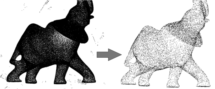
fig__Point_set_processing_3figintroduction Point set processing. Left: 275K points sampled on the statue of an elephant with a Minolta laser scanner. Right: point set after outlier removal, denoising and simplification to 17K points.
In the context of surface reconstruction we can position the elements of this component along the common surface reconstruction pipeline (fig__Point_set_processing_3figpipeline) which involves the following steps:
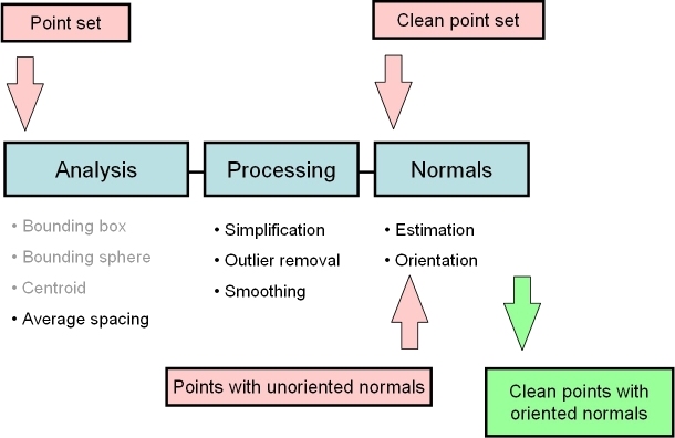
fig__Point_set_processing_3figpipeline Point set processing pipeline for surface reconstruction. The algorithms listed in gray are available from other CGAL components (bounding volumes and principal component analysis).
The algorithms of this component take as input parameters ranges of 3D points, or of 3D points with normals. They can be adapted to the user's data structures and make extensive use of named parameters and of property maps:
This API was introduced in CGAL 4.12. Please refer to the dedicated section on how to upgrade from the outdated API.
Named parameters are used to deal with optional parameters. The page Named Parameters explains the rationale and API in general. The page Named Parameters for Point Set Processing describes their usage and provides a list of the parameters that are used in this package.
The property maps are used to access the point or normal information from the input data, so as to let the user decide upon the implementation of a point with normal. The latter can be represented as, e.g., a class derived from the CGAL 3D point, or as a std::pair<Point_3<K>, Vector_3<K>>, or as a boost::tuple<..,Point_3<K>, ..., Vector_3<K> >.
The following classes described in Chapter PkgPropertyMap provide property maps for the implementations of points with normals listed above:
Identity_property_map<T>First_of_pair_property_map<Pair> and Second_of_pair_property_map<Pair>Nth_of_tuple_property_map<N, Tuple>Identity_property_map<Point_3> is the default value of the position property map expected by all functions in this component.
See below examples using pair and tuple property maps.
Users of this package may use other types to represent positions and normals if they implement the corresponding property maps.
Points and normals can even be stored in separate containers and accessed by their index, as any built-in vector is also a property map.
File Point_set_processing_3/grid_simplify_indices.cpp
The current API based on ranges and named parameters was introduced in CGAL 4.12. The old API that used pairs of iterators along with usual C++ parameters (with some default values and overloads to handle optional parameters) has been removed in CGAL 5.0.
Translating your pre-CGAL 4.12 code using Point Set Processing to the current API is easy. For example, consider this code using the old API:
The pair of iterators is replaced by a range and the optional parameters (than can be deduced automatically in simple cases) are moved to the end of the function in a single named parameter object (see Named Parameters). The code translated to the current API becomes:
Please refer to the Reference Manual for the detailed API of the Point Set Processing functions.
CGAL provides functions to read and write sets of points or sets of points with normals from the following file formats:
x y z per line or three point coordinates and three normal vector coordinates x y z nx ny nz per line)The following functions are available:
read_xyz_points()read_off_points()read_ply_points()read_las_points()write_xyz_points()write_off_points()write_ply_points()write_las_points()All of these functions (with the exception of the LAS format) can read and write either points alone or points with normals (depending on whether the normal_map is provided by the user or not).
Note that the PLY format handles both ASCII and binary formats. In addition, PLY and LAS are extensible formats that can embed additional properties. These can also be read by CGAL (see Section Points With Properties).
The following example reads a point set from an input file and writes it to a file, both in the XYZ format. Positions and normals are stored in pairs and accessed through property maps.
File Point_set_processing_3/read_write_xyz_point_set_example.cpp
PLY files are designed to embed an arbitrary number of additional attributes. More specifically, point sets may contain visibility vectors, RGB colors, intensity, etc. As it is not possible to provide dedicated functions to every possible combination of PLY properties, CGAL provides a simple way to read PLY properties and store them in any structure the user needs. Handling of LAS files works similarly with the difference that the property names and types are fixed and defined by the LAS standard.
Functions read_ply_points_with_properties() and read_las_points_with_properties() allow the user to read any property needed. The user must provide a set of property handlers that are used to instantiate number types and complex objects from PLY/LAS properties. This handlers are either:
Output functions write_ply_points_with_properties() and write_las_points_with_properties() work similarly.
The following example shows how to call write_ply_points_with_properties() to write a point set with points, RGB colors and intensity. Notice that in order to write a complex object, users need to provide an overload of CGAL::Output_rep.
File Point_set_processing_3/write_ply_points_example.cpp
The following example shows how to call read_ply_points_with_properties() to read a point set with points, normals, RGB colors and intensity and stores these attributes in a user-defined container.
File Point_set_processing_3/read_ply_points_with_colors_example.cpp
The following example shows how to call read_las_points_with_properties() to read a point set with points and RGBI colors and stores these attributes in a user-defined container.
File Point_set_processing_3/read_las_example.cpp
Function compute_average_spacing() computes the average spacing of all input points to their k nearest neighbor points, k being specified by the user. As it provides an order of a point set density, this function is used downstream the surface reconstruction pipeline to automatically determine some parameters such as output mesh sizing for surface reconstruction.
The following example reads a point set in the xyz format and computes the average spacing. Index, position and color are stored in a tuple and accessed through property maps.
File Point_set_processing_3/average_spacing_example.cpp
Note that other functions such as centroid or bounding volumes are found in other CGAL components:
Point sets are often used to sample objects with a higher dimension, typically a curve in 2D or a surface in 3D. In such cases, finding the scale of the objet is crucial, that is to say finding the minimal number of points (or the minimal local range) such that the subset of points has the appearance of a curve in 2D or a surface in 3D [2].
CGAL provides two functions that automatically estimate the scale of a 2D point set sampling a curve or a 3D point set sampling a surface:
Functions such as grid_simplify_point_set() require a range scale while jet_estimate_normals(), remove_outliers() or vcm_estimate_normals() are examples of functions that accepts both a K neighbor scale or a range scale.
In some specific cases, the scale of a point set might not be homogeneous (for example if the point set contains variable noise). CGAL also provides two functions that automatically estimate the scales of a point set at a set of user-defined query points:
The 4 functions presented here work both with 2D points and 3D points and they shouldn't be used if the point sets do not sample a curve in 2D or a surface in 3D.
The following example reads a 3D point set in the xyz format and:
File Point_set_processing_3/scale_estimation_example.cpp
This second example generates a 2D point set sampling a circle with variable noise. It then estimates the scale at 3 different query points in the domain.
File Point_set_processing_3/scale_estimation_2d_example.cpp
CGAL provides two functions as wrapper for the thirdpartyOpenGR library [8], and two functions as wrapper for the thirdpartylibpointmatcher library :
CGAL::OpenGR::compute_registration_transformation() computes the registration of one point set w.r.t. another in the form of a CGAL::Aff_transformation_3 object, using the Super4PCS algorithm [9];CGAL::OpenGR::register_point_sets() computes the registration of one point set w.r.t. another and directly aligns it to it;CGAL::pointmatcher::compute_registration_transformation() computes the registration of one point set w.r.t. another in the form of a CGAL::Aff_transformation_3 object, using the ICP (Iterative Closest Point) algorithm;CGAL::pointmatcher::register_point_sets() computes the registration of one point set w.r.t. another and directly aligns it to it.The following example reads two point sets and aligns them using the thirdpartyOpenGR library, using the Super4PCS algorithm:
File Point_set_processing_3/registration_with_OpenGR.cpp
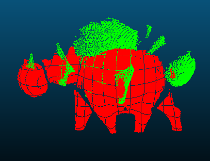
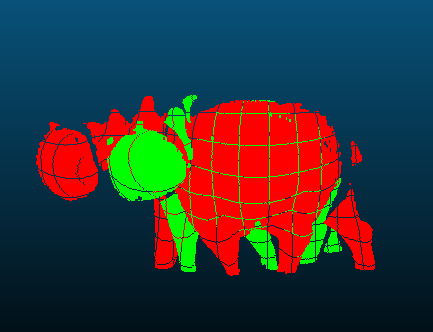
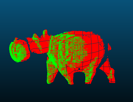
fig__Point_set_processing_3tableRegistrationRegistration_visualization_table demonstrates visualization of a scan data before and after different registration methods are applied, including the OpenGR registration method. To obtain the results for OpenGR registration in the visualization table, above-mentioned example was used.
Input clouds are sub-sampled prior exploration, to ensure fast computations. Super4PCS has a linear complexity w.r.t. the number of input samples, allowing to use larger values than 4PCS. Simple geometry with large overlap can be matched with only 200 samples. However, with Super4PCS, smaller details can be used during the process by using up to thousands of points. There is no theoretical limit to this parameter; however, using too large values leads to very a large congruent set, which requires more time and memory to be explored.
Using a large number of samples is recommended when:
Note that Super4PCS is a global registration algorithm, which finds a good approximate of the rigid transformation aligning two clouds. Increasing the number of samples in order to get a fine registration is not optimal: it is usually faster to use fewer samples, and refine the transformation using a local algorithm, like the ICP, or its variant SparseICP.
This parameter controls the registration accuracy: setting a small value means that the two clouds need to be very close to be considered as well aligned. It is expressed in scene units.
A simple way to understand its impact is to consider the computation of the Largest Common Pointset (LCP), the metric used to verify how aligned the clouds are. For each transformation matrix produced by Super4PCS, OpenGR computes the LCP measure by considering a shell around the reference cloud, and count the percentage of points of the target cloud lying in the shell. The thickness of the shell is defined by the parameter delta (accuracy).
Using too wide values will slow down the algorithm by increasing the size of the congruent set, while using to small values prevents to find a solution. This parameter impacts other steps of the algorithm, see the paper [9] for more details.
This parameter sets an angle threshold above which two pairs of points are discarded as candidates for matching. It is expressed in degrees.
The default value is 90° (no filtering). Decreasing this value allows to decrease the computation time by being more selective on candidates. Using too small values might result in ignoring candidates that should indeed have been matched and may thus result in a quality decrease.
Ratio of expected overlap between the two point sets: it is ranging between 0 (no overlap) to 1 (100% overlap).
The overlap parameter controls the size of the basis used for registration, as shown below:

fig__Point_set_processing_3figOpenGR_parameter_overlap The effect of varying overlap parameter on the size of the basis used for registration. The overlap is smaller for left (a) than right (b).
Usually, the larger the overlap, the faster the algorithm. When the overlap is unknown, a simple way to set this parameter is to start from 100% overlap, and decrease the value until obtaining a good result. Using too small values will slow down the algorithm, and reduce the accuracy of the result.
Maximum number of seconds after which the algorithm stops. Super4PCS explores the transformation space to align the two input clouds. Since the exploration is performed randomly, it is recommended to use a large time value to explore the whole space.
The following example reads two point sets and aligns them using the thirdpartylibpointmatcher library, using the ICP algorithm. It also shows how to customize ICP algorithm by using possible configurations:
File Point_set_processing_3/registration_with_pointmatcher.cpp
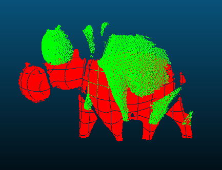
fig__Point_set_processing_3tableRegistrationRegistration_visualization_table demonstrates visualization of a scan data before and after different registration methods are applied, including the PointMatcher registration method. To obtain the results for PointMatcher registration in the visualization table, above-mentioned example was used.
The chain of filters to be applied to the point cloud. The point cloud is processed into an intermediate point cloud with the given chain of filters to be used in the alignment procedure. The chain is organized with the forward traversal order of the point set filters range.
The chain of point set filters are applied only once at the beginning of the ICP procedure, i.e., before the first iteration of the ICP algorithm.
The filters can have several purposes, including but not limited to:
In registration, there are two point clouds in consideration, one of which is the reference point cloud while the other one is the point cloud to register. The point set filters corresponds to readingDataPointsFilters configuration module of thirdpartylibpointmatcher library while it corresponds to the referenceDataPointsFilters for the other point cloud. The filters should be chosen and set from possible components of those configuration modules.
The method used for matching (linking) the points from to the points in the reference cloud.
Corresponds to matcher configuration module of thirdpartylibpointmatcher library. The matcher should be chosen and set from possible components of the matcher configuration module. See libpointmatcher documentation for possible configurations.
The chain of filters to be applied to the matched (linked) point clouds after each processing iteration of the ICP algorithm to remove the links which do not correspond to true point correspondences. The outliers are rejected. Points with no link are ignored in the subsequent error minimization step. The chain is organized with the forward traversal order of the outlier filters range.
Corresponds to outlierFilters configuration module of thirdpartylibpointmatcher library. The filters should be chosen and set from possible components of the outlierFilters configuration module. See libpointmatcher documentation for possible configurations.
The error minimizer that computes a transformation matrix such as to minimize the error between the point sets.
Corresponds to errorMinimizer configuration module of thirdpartylibpointmatcher library. The error minimizer should be chosen and set from possible components of the errorMinimizer configuration module. See libpointmatcher documentation for possible configurations.
The inspector allows to log data at different steps for analysis. Inspectors typically provide deeper scrutiny than the logger.
Corresponds to inspector configuration module of thirdpartylibpointmatcher library. The inspector should be chosen and set from possible components of the inspector configuration module. See libpointmatcher documentation for possible configurations.
The method for logging information regarding the registration process outputted by thirdpartylibpointmatcher library. The logs generated by CGAL library does not get effected by this configuration.
Corresponds to logger configuration module of thirdpartylibpointmatcher library. The logger should be chosen and set from possible components of the logger configuration module. See libpointmatcher documentation for possible configurations.
The affine transformation that is used as the initial transformation for the reference point cloud.
The following example reads two point sets and aligns them by using both thirdpartyOpenGR and thirdpartylibpointmatcher libraries, respectively. It depicts a use case where a coarse estimation of a registration transformation is done using the Super4PCS algorithm. Then, a fine registration from this coarse registration using the ICP algorithm.
File Point_set_processing_3/registration_with_opengr_pointmatcher_pipeline.cpp
fig__Point_set_processing_3tableRegistrationRegistration_visualization_table demonstrates visualization of a scan data before and after different registration methods are applied, including the pipeline of OpenGR and PointMatcher registration methods. To obtain the results for the pipeline of OpenGR and PointMatcher registration methods in the visualization table, above-mentioned example was used.
| Scan 1 | Scan 1 (possibly transformed, green) and Scan 2 (the reference, red) | |
|---|---|---|
| Unregistered | 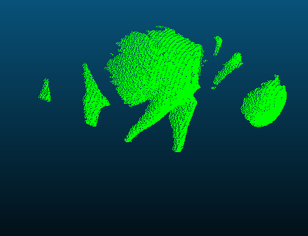
| 
|
| Registered using OpenGR | 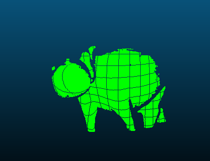
| 
|
| Registered using PointMatcher | 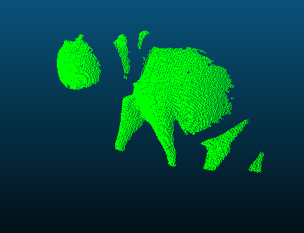
| 
|
| Registered using OpenGR+PointMatcher Pipeline | 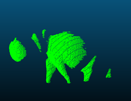
| 
|
fig__Point_set_processing_3tableRegistrationRegistration_visualization_table Visualization of registered hippo scans with different registration methods. Two scans are used: red as the reference, green as the one for which the transformation is computed and applied. To obtain the results, the example code given in OpenGR Example , PointMatcher Example , OpenGR/PointMatcher Pipeline Example were applied, respectively. The parameters of the algorithms used to obtain those results are not optimized for the shown scans; therefore, better parameter choice might result in better results in terms of registration accuracy for each algorithm individually.
Function remove_outliers() deletes a user-specified fraction of outliers from an input point set. More specifically, it sorts the input points in increasing order of average squared distances to their nearest neighbors and deletes the points with largest value. The user can either specify a fixed number of nearest neighbors or a fixed spherical neighborhood radius.
The following example reads a point set and removes 5% of the points. It uses the Identity_property_map<Point_3> property map (optional as it is the default position property map of all functions in this component.)
File Point_set_processing_3/remove_outliers_example.cpp
Four simplification functions are devised to reduce an input point set.
Function random_simplify_point_set() randomly deletes a user-specified fraction of points from the input point set. This algorithm is fast.
Function grid_simplify_point_set() considers a regular grid covering the bounding box of the input point set, and clusters all points sharing the same cell of the grid by picking as representant one arbitrarily chosen point. This algorithm is slower than random_simplify_point_set().
Function hierarchy_simplify_point_set() provides an adaptive simplification of the point set through local clusters [11]. The size of the clusters is either directly selected by the user or it automatically adapts to the local variation of the point set.
Function wlop_simplify_and_regularize_point_set() not only simplifies, but also regularizes downsampled points. This is an implementation of the Weighted Locally Optimal Projection (WLOP) algorithm [4].
The following example reads a point set and simplifies it by clustering.
File Point_set_processing_3/grid_simplification_example.cpp
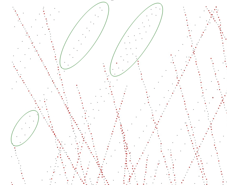
fig__Point_set_processing_3figgrid_simplification Point set simplification through grid-based clustering. Removed points are depicted in red. Notice how low-density areas (in green) are not simplified.
The following example reads a point set and produces a set of clusters.
File Point_set_processing_3/hierarchy_simplification_example.cpp
The hierarchy simplification algorithm recursively split the point set in two until each cluster's size is less than the parameter size.

fig__Point_set_processing_3figHierarchy_simplification_size Input point set and hierarchy simplification with different size parameter: \(10\), \(100\) and \(1000\). In the 3 cases, var_max \(=1/3\).
In addition to the size parameter, a variation parameter allows to increase simplification in monotonous regions. For each cluster, a surface variation measure is computed using the sorted eigenvalues of the covariance matrix:
\[ \sigma(p) = \frac{\lambda_0}{\lambda_0 + \lambda_1 + \lambda_2}. \]
This function goes from \(0\) if the cluster is coplanar to \(1/3\) if it is fully isotropic. If a cluster's variation is above var_max, it is split. If var_max is equal to \(1/3\), this parameter has no effect and the clustering is regular on the whole point set.

fig__Point_set_processing_3figHierarchical_clustering_var_max Input point set and hierarchy simplification with different var_max parameter: \(0.00001\), \(0.001\) and \(0.1\). In the 3 cases, size \(=1000\).
The following example reads a point set, simplifies and regularizes it by WLOP.
File Point_set_processing_3/wlop_simplify_and_regularize_point_set_example.cpp

fig__Point_set_processing_3figsimplification_comparison Comparison for three simplification methods: Left: Random simplification result. Middle: Grid simplification result. Right: WLOP simplification result.
Computing density weights for each point is an optional preprocessing. For example, as shown in the following figure, when require_uniform_sampling is set to false, WLOP preserves the intrinsic non-uniform sampling of the original points; if require_uniform_sampling is set to true, WLOP is resilient to non-uniform sampling and generates sample points with more uniform distribution, at the expense of computational time.

fig__Point_set_processing_3figWLOP_parameter_density Comparison between with and without density: Left: input. Middle: require_uniform_sampling = false. Right: require_uniform_sampling=true.
Usually, the neighborhood of sample points should include at least two rings of neighboring sample points. Using a small neighborhood size may not be able to generate regularized result, while using big neighborhood size will make the sample points shrink into the interior of the local surface (under-fitting). The function will use a neighborhood size estimation if this parameter value is set to default or smaller that zero.

fig__Point_set_processing_3figWLOP_parameter_neighborhood_size Comparison between different sizes of neighbor radius.
A parallel version of WLOP is provided and requires the executable to be linked against the Intel TBB library. To control the number of threads used, the user may use the tbb::task_scheduler_init class. See the TBB documentation for more details. We provide below a speed-up chart generated using the parallel version of the WLOP algorithm. The machine used is a PC running Windows 7 64-bits with a 4-core i7-4700HQ@2.40GHz CPU with 8GB of RAM.
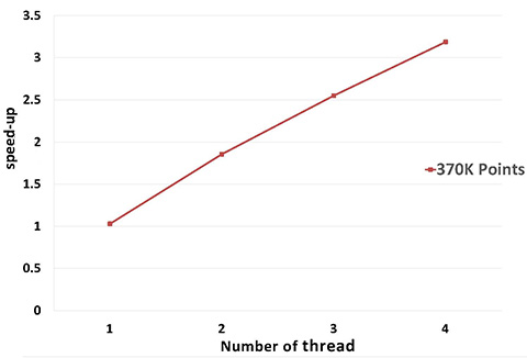
fig__Point_set_processing_3figWLOP_parallel_performance Parallel WLOP speed-up, compared to the sequential version of the algorithm.
Two smoothing functions are devised to smooth an input point set.
Function jet_smooth_point_set() smooths the input point set by projecting each point onto a smooth parametric surface patch (so-called jet surface) fitted over its nearest neighbors.
Function bilateral_smooth_point_set() smooths the input point set by iteratively projecting each point onto the implicit surface patch fitted over its nearest neighbors. Bilateral projection preserves sharp features according to the normal (gradient) information. Normals are thus required as input. For more details, see section 4 of [5].
For both functions, the user can either specify a fixed number of nearest neighbors or a fixed spherical neighborhood radius.
The following example generates a set of 9 points close to the xy plane and smooths them using 8 nearest neighbors:
File Point_set_processing_3/jet_smoothing_example.cpp
The following example reads a set of points with normals and smooths them via bilateral smoothing:
File Point_set_processing_3/bilateral_smooth_point_set_example.cpp

fig__Point_set_processing_3figsmoothing_comparison Comparison for two smoothing methods: Left: Input, 250K points, normal-color mapping. Middle: Jet smoothing result, 197 seconds. Right: Bilateral smoothing result, 110 seconds.
Performance: A parallel version of bilateral smoothing is provided and requires the executable to be linked against the Intel TBB library. The number of threads used is controlled through the tbb::task_scheduler_init class. See the TBB documentation for more details. We provide below a speed-up chart generated using the parallel version of the bilateral smoothing algorithm. The machine used is a PC running Windows 7 64-bits with a 4-core i7-4700HQ@2.40GHz CPU with 8GB of RAM.
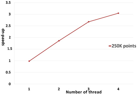
fig__Point_set_processing_3Bilateral_smoothing_parallel_performance Parallel bilateral smoothing speed-up, compared to the sequential version of the algorithm.
Assuming a point set sampled over an inferred surface S, two functions provide an estimate of the normal to S at each point. The result is an unoriented normal vector for each input point.
Function jet_estimate_normals() estimates the normal direction at each point from the input set by fitting a jet surface over its nearest neighbors. The default jet is a quadric surface. This algorithm is well suited to point sets scattered over curved surfaces.
Function pca_estimate_normals() estimates the normal direction at each point from the set by linear least squares fitting of a plane over its nearest neighbors. This algorithm is simpler and faster than jet_estimate_normals().
Function vcm_estimate_normals() estimates the normal direction at each point from the set by using the Voronoi Covariance Measure of the point set. This algorithm is more complex and slower than the previous algorithms. It is based on the article [10].
For these three functions, the user can either specify a fixed number of nearest neighbors or a fixed spherical neighborhood radius.
Function mst_orient_normals() orients the normals of a set of points with unoriented normals using the method described by Hoppe et al. in Surface reconstruction from unorganized points [3]. More specifically, this method constructs a Riemannian graph over the input points (the graph of the nearest neighbor points) and propagates a seed normal orientation within a minimum spanning tree computed over this graph. The result is an oriented normal vector for each input unoriented normal, except for the normals which cannot be successfully oriented.
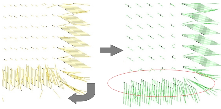
fig__Point_set_processing_3figmst_orient_normals Normal orientation of a sampled cube surface. Left: unoriented normals. Right: orientation of right face normals is propagated to bottom face.
The following example reads a point set from a file, estimates the normals through PCA (either over the 18 nearest neighbors or using a spherical neighborhood radius of twice the average spacing) and orients the normals:
File Point_set_processing_3/normals_example.cpp
The function edge_aware_upsample_point_set() generates a denser point set from an input point set. This has applications in point-based rendering, hole filling, and sparse surface reconstruction. The algorithm can progressively upsample the point set while approaching the edge singularities. See [5] for more details.
The following example reads a point set from a file, upsamples it to get a denser result.
File Point_set_processing_3/edge_aware_upsample_point_set_example.cpp
This parameter controls where the new points are inserted. Larger values of edge-sensitivity give higher priority to inserting points along the sharp features. For example, as shown in the following figure, high value is preferable when one wants to insert more points on sharp features, where the local gradient is high, e.g., darts, cusps, creases and corners. In contrast, points are evenly inserted when edge_sensitivity is set to 0. The range of possible value is [0, 1].

fig__Point_set_processing_3figUpsample_edge_sensitivity Upsampling for different edge-sensitivity parameter values. The input containing 850 points is upsampled to 1,500 points in all cases depicted.
This parameter controls the preservation of sharp features.

fig__Point_set_processing_3figUpsample_sharpness_angle Upsampling for different sharpness_angle parameter values. The input containing 850 points is upsampled to 425K points in all cases depicted.
Usually, the neighborhood of sample points should include at least one ring of neighboring sample points. Using small neighborhood size may not be able to insert new points. Using big neighborhood size can fill small holes, but points inserted on the edges could be irregular. The function will use a neighborhood size estimation if this parameter value is set to default or smaller than zero.

fig__Point_set_processing_3figupsample_neighborhood_size Comparison between different sizes of neighbor radius.
Function vcm_is_on_feature_edge() indicates if a points belong to a feature edges of the point set using its Voronoi Covariance Measure. It is based on the article [10].
It first computes the VCM of the points set using compute_vcm(). Then, it estimates which points belong to a sharp edge by testing if a ratio of eigenvalues is greater than a given threshold.
The following example reads a point set from a file, estimates the points that are on sharp edges:
File Point_set_processing_3/edges_example.cpp
The function structure_point_set() generates a structured version of the input point set assigned to a set of planes. Such an input can be produced by a shape detection algorithm (see Shape Detection Reference). Point set structuring is based on the article [7].
This algorithm is well suited to point sets sampled on surfaces with planar sections and sharp edges.
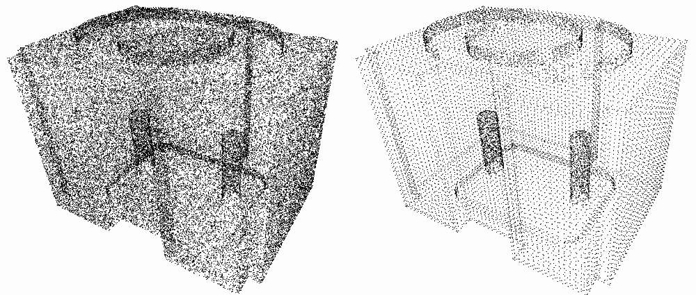
fig__Point_set_processing_3figstructuring Point set structuring. Left: input raw point set. Right: structured point set.
Structure information of points can be used to perform feature preserving reconstruction (see Advancing Front Surface Reconstruction for example). More specifically, the class storing a point set with structure provides the user with a method Point_set_with_structure::facet_coherence() that estimates if a triplet of points form a coherent facet.
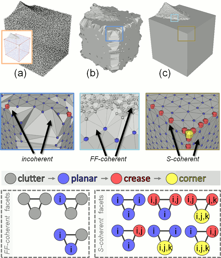
fig__Point_set_processing_3figstructuring_coherence (a) Input point set (and structured output); (b) output with many incoherent facets; (c) output with all facets coherent. i, j and k each corresponds to a primitive index.
The following example applies shape detection followed by structuring to a point set:
File Point_set_processing_3/structuring_example.cpp
Several functions of this package provide a callback mechanism that enables the user to track the progress of the algorithms and to interrupt them if needed. A callback, in this package, is an instance of std::function<bool(double)> that takes the advancement as a parameter (between 0. when the algorithm begins to 1. when the algorithm is completed) and that returns true if the algorithm should carry on, false otherwise. It is passed as a named parameter with an empty function as default.
Algorithms that support this mechanism are detailed in the Reference Manual, along with the effect that an early interruption has on the output.
The following example defines a callback that displays the name of the current algorithm along with the progress (as a percentage) updated every \(1/10th\) of a second. While the algorithm is running, the console output will typically look like this:
Thanks to the carriage return character \r, the lines are overwritten and the user sees the percentage increasing on each line.
File Point_set_processing_3/callback_example.cpp
Pierre Alliez and Laurent Saboret contributed the initial component. Nader Salman contributed the grid simplification. Started from GSoC'2013, three new algorithms were implemented by Shihao Wu and Clément Jamin: WLOP, bilateral smoothing and upsampling. Started from GSoC'2014, Jocelyn Meyron with the help of Quentin Mérigot introduced the computation of the Voronoi covariance measure of a point set, as well as the normal and feature edge estimation functions based on it. Florent Lafarge with the help of Simon Giraudot contributed the point set structuring algorithm. Started from GSoC'2019, Necip Fazil Yildiran with the help of Nicolas Mellado and Simon Giraudot introduced the wrappers for OpenGR and PointMatcher libraries that perform registration on two point sets.